決定木から始める機械学習

# 表形式のデータを操作するためのライブラリ
import pandas as pd

# 機械学習用ライブラリsklearn
from sklearn.model_selection import train_test_split
from sklearn.tree import DecisionTreeClassifier
from sklearn.metrics import accuracy_score
from sklearn.tree import export_graphviz

# その他
import category_encoders

# グラフ描画ライブラリ
from graphviz import Source
import matplotlib.pyplot as plt
%matplotlib inline

---

クイズ

以下のコードを実行してincome_dfに格納されるデータは，ある年にアメリカで実施された国勢調査のデータである．

# データの読み込み
income_df = pd.read_table("https://archive.ics.uci.edu/ml/machine-learning-databases/adult/adult.data", sep=',', header=None)

# 列名（特徴）に名前を付ける
income_df.columns = ['age', 'workclass', 'fnlwgt', 'education', 'education-num', 'marital-status', 'occupation', 
                     'relationship', 'race', 'sex', 'capital-gain', 'capital-loss', 'hours-per-week', 'native-country', 'income']

# データ表示（先頭5件）
income_df.head()

	age	workclass	fnlwgt	education	education-num	marital-status	occupation	relationship	race	sex	capital-gain	capital-loss	hours-per-week	native-country	income
0	39	State-gov	77516	Bachelors	13	Never-married	Adm-clerical	Not-in-family	White	Male	2174	0	40	United-States	<=50K
1	50	Self-emp-not-inc	83311	Bachelors	13	Married-civ-spouse	Exec-managerial	Husband	White	Male	0	0	13	United-States	<=50K
2	38	Private	215646	HS-grad	9	Divorced	Handlers-cleaners	Not-in-family	White	Male	0	0	40	United-States	<=50K
3	53	Private	234721	11th	7	Married-civ-spouse	Handlers-cleaners	Husband	Black	Male	0	0	40	United-States	<=50K
4	28	Private	338409	Bachelors	13	Married-civ-spouse	Prof-specialty	Wife	Black	Female	0	0	40	Cuba	<=50K

データ中の列名（特徴量）の意味は以下の通りである：

• age: 年齢（整数）

• workclass: 雇用形態（公務員，会社員など）

• fnlwgt: 使わない

• education: 学歴

• education-num: 使わない

• marital-status: 婚姻状態

• occupation: 職業

• relationship: 家族内における役割

• race: 人種

• sex: 性別

• capital-gain: 使わない

• capital-loss: 使わない

• hours-per-week: 週あたりの労働時間（整数値）

• native-country: 出身国

• income: 年収（50Kドル以上，50Kドル未満の二値）

このデータに対して決定木アルゴリズムを適用して，ある人物が年間収入が50Kドル以上か未満かを分類する機械学習モデルを構築したい．

Q1: ヒストグラム

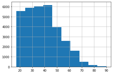
機械学習モデルを構築する前に，income_dfデータに含まれる調査対象者の年齢の分布を知りたい． 年齢に関するヒストグラム（階級数は10）を作成せよ．

※ ヒント: ヒストグラムの作成にはpandas.series.hist関数を用いるとよい（参考）

income_df['age'].hist(bins=10)

<AxesSubplot:>

Q2: 出現頻度

機械学習モデルを構築する前に，income_dfデータに含まれる性別，年収の分布を知りたい． 性別（男，女），年収（50K以上，50K未満）について，属性値に対応する人数を求めよ．

※ ヒント: 要素の出現頻度を求めるにはpandas.series.value_countsメソッドを用いるとよい（参考）

income_df['sex'].value_counts()

 Male      21790
 Female    10771
Name: sex, dtype: int64

income_df['income'].value_counts()

 <=50K    24720
 >50K      7841
Name: income, dtype: int64

Q3: データの集約

income_dfデータを集約し，学歴ごとに年間収入クラスの内訳（割合）を調べよ．

※ ヒント: pandasのcrosstab関数を使う（タイタニックの例でも使ったので，確認してみよう）

pd.crosstab(income_df['education'], income_df['income'], normalize='index')

income	<=50K	>50K
education
10th	0.933548	0.066452
11th	0.948936	0.051064
12th	0.923788	0.076212
1st-4th	0.964286	0.035714
5th-6th	0.951952	0.048048
7th-8th	0.938080	0.061920
9th	0.947471	0.052529
Assoc-acdm	0.751640	0.248360
Assoc-voc	0.738784	0.261216
Bachelors	0.585247	0.414753
Doctorate	0.259080	0.740920
HS-grad	0.840491	0.159509
Masters	0.443413	0.556587
Preschool	1.000000	0.000000
Prof-school	0.265625	0.734375
Some-college	0.809765	0.190235

Q4: 学習のためのデータ分割

income_dfデータに決定木アルゴリズムを適用するために，データを7:3に分割し，7割のデータを学習用データ（income_train_df），3割のデータを評価用データ（income_test_df）としなさい．

# データを学習用（70%）と評価用（30%）に分割する
income_train_df, income_test_df = train_test_split(
                                income_df,
                                test_size=0.3,
                                random_state=1,
                                stratify=income_df.income)

Q5: 決定木の構築

以下は，「年齢」「雇用形態」「学歴」「婚姻の有無」「職業」「家族内における役割」「人種」「性別」「週あたりの労働時間」「出身国」の属性に着目して，income_dfデータから年収カテゴリを予測する決定木を構築するコードである． # ---------- の間を埋めてコードを完成させなさい．

# 注目する属性
target_features = ['age', 'workclass', 'education', 'marital-status', 'occupation', 
                   'relationship', 'race', 'sex', 'hours-per-week', 'native-country']

# 数値に変換したいカテゴリ変数
encoded_features = ['education', 'workclass', 'marital-status', 'relationship', 'occupation', 'native-country', 'race', 'sex']

# カテゴリ変数を数値情報に変換する
encoder = category_encoders.OneHotEncoder(cols=encoded_features, use_cat_names=True)
encoder.fit(income_train_df[target_features])

# ---------------------
# ここから必要なコードを埋める

# 予測に用いる年収情報以外のすべての指標をX_trainに
X_train = income_train_df[target_features]

# カテゴリ変数を数値情報に変換
X_train = encoder.transform(X_train)

# y_trainは年収クラスをあらわす指標
y_train = income_train_df.income

# 学習器の定義（決定木を使う）
model = DecisionTreeClassifier(criterion='entropy',
                               max_depth=5)

# ここまで必要なコードを埋める
# ---------------------

# 学習用データを使って学習
model.fit(X_train, y_train)

DecisionTreeClassifier(criterion='entropy', max_depth=5)

Q6: 決定木における各属性の寄与度

構築した決定木モデル（model）を用いて，年収（income）の分類における各属性（列）の寄与度を表示しなさい． なお，寄与度がゼロのものは表示しなくてよい．

for feature, importance in zip(X_train.columns, model.feature_importances_):
    if importance > 0:
        print("{}\t{}".format(feature, importance))

age	0.0894604682456178
workclass_ State-gov	0.000640985686209342
education_ Bachelors	0.06141563902135156
education_ Some-college	0.006168600381132655
education_ Prof-school	0.003625407861733974
education_ HS-grad	0.00881490359411402
education_ Masters	0.010774717032624306
marital-status_ Married-civ-spouse	0.5943231227829802
occupation_ Prof-specialty	0.07941724495727506
occupation_ Exec-managerial	0.0643690097067649
occupation_ Protective-serv	0.0011395499411790816
sex_ Male	0.0020402074457221034
sex_ Female	0.0020803940555122083
hours-per-week	0.07499207892598281
native-country_ Portugal	0.0007376703617999955

Q7: 決定木の再構築

Q6の結果をもとに年収分類に寄与する特徴量を（最大5つ）特定し，その特徴量のみを用いて再度決定木モデルを構築しなさい． その際，あまり木が深くならないよう調整し，できる限りシンプルなモデルになるようにすること．

target_features = ['age', 'education', 'marital-status', 'occupation', 'hours-per-week']
encoded_features = ['education', 'marital-status', 'occupation']

encoder = category_encoders.OneHotEncoder(cols=encoded_features, use_cat_names=True)
encoder.fit(income_train_df[target_features])

X_train = income_train_df[target_features]
X_train = encoder.transform(X_train)
y_train = income_train_df.income

# 学習
model = DecisionTreeClassifier(criterion='entropy', max_depth=3)
model.fit(X_train, y_train)

DecisionTreeClassifier(criterion='entropy', max_depth=3)

Source(export_graphviz(
    model, out_file=None,
    feature_names=X_train.columns,
    class_names=['<=50K', '>50K'],
    proportion=True,
    filled=True, rounded=True # 見た目の調整
))